[데이터 사이언스] Mining max patterns & closed patterns
in CS Review on DataScience
Frequent pattern이 너무 많아서 그 대신 max pattern이나 closed pattern과 같은 좀 더 엄격한 룰을 적용한 패턴을 마이닝하는 것이 보완책으로 제안되었다.
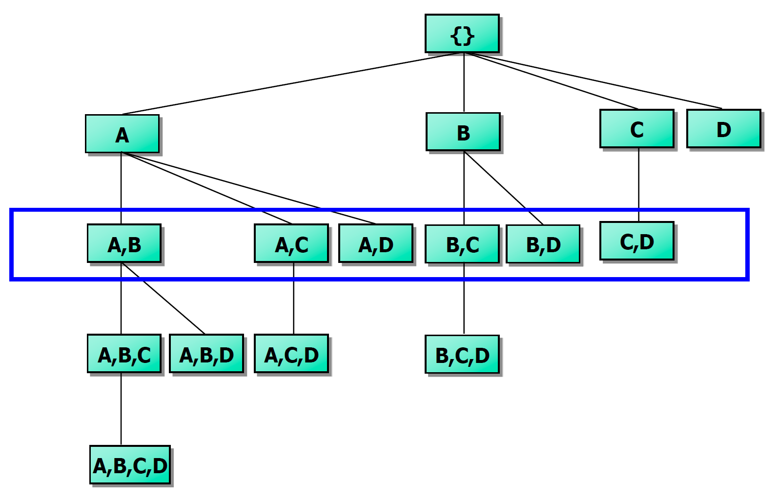
MaxMiner: Mining Max-patterns
Max pattern은 더 늘릴 게 없는 frequent pattern이다. 즉, frequent super pattern이 없는 상태를 말한다.
Apriori 알고리즘을 기반으로, max pattern만을 효과적으로 구하기 위한 방법으로 MaxMiner가 제시되었다.
첫 번째 scan에서 frequent item들을 찾고 오름차순(frequency 기준)으로 정렬한다. ex) A, B, C, D, E 순이라면, E가 제일 빈번함
두 번째 scan에서 2-itemsets와 potential max-patterns의 support를 구한다. 만들 때, ascending order로 정렬한 순서를 지켜서 생성해주어야 한다. 위의 예시에서 BC는 있어도 CB는 없다!! Ascending order를 지켜서 생성할 때마다 해당 아이템으로 만들 수 있는 max-pattern의 후보(potential max-pattern)를 추가한다.
Ascending order를 지켜서 생성하고 potential max-pattern을 추가해준다고 했는데 어떻게 이뤄질까? Set-enumeration tree를 이용하면 된다!! Frequency 순서대로 진행하며 만들 수 있는 pattern을 계속 만들다가 마지막 leaf node에 위치한 것이 potential max pattern이 되는 것이다.
ex) {BC, BD, BE}라면 potential max-patterns는 BCDE 이런식으로 구해서 만약 BCDE가 frequent하다면, 그의 부분집합도 모두 freqeunt하다. 즉, BCD, BDE, CDE를 검증할 필요가 없어진다. 또한, AC가 frequent하지 않다면, ABC는 검증할 필요가 없어진다.
결과적으로 이후의 단계에서 많은 후보를 줄일 수 있게 된다.
CLOSET: Mining Closed-patterns
Closed pattern은 frequent pattern인 동시에 그와 같은 support를 갖는 super pattern이 없는 것이다. CLOSET은 FP-tree를 사용해서 frequent pattern을 찾는다.
F-list를 그대로 사용하는데 이는 descending order라는 것을 알고 있다. 마찬가지로 divide and conquer로 f-list의 제일 작은 frequency부터 패턴을 따져주면 된다.
Closed pattern을 찾는 naive한 approach는 모든 frequent itemset을 찾고 그들의 superset과 support가 같은 것은 다 drop하면 된다. 이런 방식은 cost가 좀 있기 때문에 다른 방식을 찾아보아야 한다!!
FP-growth를 통해서 cfa라는 frequent pattern을 찾았는데 cfa를 갖고 있는 모든 트랜잭션이 d를 가지고 있다면 cfa와 cfad의 frequency가 같다는 것을 알 수 있고, cfa는 적어도 closed pattern이 아니라는 것을 알 수 있다.
CHARM: Mining by Exploring Vertical Data Format
Vertical Format이란 트랜잭션 관점(horizontal view)에서 보는 것이 아닌 아이템셋 관점으로 보는 것이다. 해당 아이템셋을 갖고 있는 트랜잭션을 list(tid-list)로 갖는다고 생각하면 된다.
ex) t(AB) = {T11, T25, …}
Horizontal한 format을 vertical로 바꾸기 위해 한 번 scan한다. Item 수가 transaction 수보다 훨~~~씬 적기 때문에 쉽다. 그 다음, K=1부터 K+1 itemset의 후보를 만든다. Tid-sets interaction(Minsup 넘어야 함)과 Apriori property를 이용한다. 그래서 frequent itemset이 더 이상 나오지 않을때까지 반복한다.
| itemset | TID_set |
|---|---|
| I1 | {T100, T400, T500, T700, T800, T900} |
| I2 | {T100, T200, T300, T400, T600, T800, T900} |
| I3 | {T300, T500, T600, T700, T800, T900} |
| I4 | {T200, T400} |
| I5 | {T100, T800} |
I1 intersection I2 = {T100, T400, T800, T900}.. 이런식으로 계산해서 2-itemset을 vertical data format으로 만들어준다. Minimum support가 2이다.
| itemset | TID_set |
|---|---|
| {I1, I2} | {T100, T400, T800, T900} |
| {I1, I3} | {T500, T700, T800, T900} |
| {I1, I4} | {T400} |
| {I1, I5} | {T100, T800} |
| {I2, I3} | {T300, T600, T800, T900} |
| {I2, I4} | {T200, T400} |
| {I2, I5} | {T100, T800} |
| {I3, I5} | {T800} |
| itemset | TID_set |
|---|---|
| {I1, I2, I3} | {T800, T900} |
| {I1, I2, I5} | {T100, T800} |
위와 같이 진행되는 것이다.
장점으로는 (k+1)-itemsets의 support를 계산하기 위해 database를 스캔하지 않아도 된다. TID-set이 자체로 support value를 지니고 있기 때문이다. 하지만 intersection에 많은 시간과 공간이 필요하다. 이를 해결하기 위해 diffset technique를 이용한다. 두 아이템셋이 등장하는 transaction id를 비교하여 차집합만 저장한다.
Mining various kinds of association rules
a. Mining multi-level association
아이템들은 주로 계층을 형성한다!! 계층이 낮을 수록 낮은 support value를 사용하는 것이 좋다. 예를 들어, Milk라는 아이템이 있고 2% milk, skim milk라는 하위 계층의 milk가 있다면 당연히 하위 계층에 낮은 support value를 적용하는 것이 당연해보인다. 그게 reduced support라고 하고 그렇지 않고 똑같이 적용하는 것이 uniform support이다. uniform support는 계층이 낮을수록 association rule에 포함되기 힘들고, 높을수록 포함되기 쉬워진다.
Redundancy Filtering
어떤 rule들은 ancestor가 있기 때문에 중복되는 경우가 있다.
milk => wheat bread (support=8%, confidence=70%)
2% milk => wheat bread (support=2%, confidence=72%)
위와 같을 때 첫 번째 rule이 두 번째 rule의 ancestor라고 한다.
Descendent rule은 descendent의 support가 ancestor의 support값과 비교하여 기대하는 값과 비슷하고, descendent의 confidence값이 ancestor의 confidence 와 비슷할 때, ‘redundant’ 하다고 한다.
b. Mining multi-dimensional association
Single-dimensional rules: 하나의 dimension이나 predicate를 갖는다.
ex) buys(X, “milk”) => buys(X, “bread”): milk->bread 처럼 buys 하나의 predicate만 사용!!Multi-dimensional rules: 2개 이상의 dimensions나 predicates를 갖는다.
- Inter-dimension association rules(no repeated predicates)
ex) age(X, “19-25”) ^ occupation(X, “student”) => buys(X, “coke”) - Hybrid-dimension association rules(repeated predicates)
ex) age(X, “19-25”) ^ buys(X, “popcorn”) => buys(X, “coke”)
- Inter-dimension association rules(no repeated predicates)
age(X, "19-25") ^ occupation(X, "student") => buys(X, "coke")
Attribute Types
위의 “19-25”, “student”, “coke”들이 attribute에 해당된다.
- Categorical Attributes: value가 유한한 양수이고 value 사이에 순서가 없다.
- Quantitative Attributes: Numeric이며 value 사이에 암시된 순서가 있으며, 이산화하거나 클러스터링 작업이 필요한데 실수형으로 하면 데이터 마이닝을 하기 쉽지 않기 때문이다. 결국 Range에 더 많이 걸리게 하기 위해서이다.
c. Mining quantitative association
1. Static discretization based on predefined concept hierarchies(data cube methods): Numeric values는 concept hierarchy를 이용하여 range(categorical value 처럼)로 바꾸고, k-predicate sets는 k 또는 k+1의 table scan이 필요하다.
ex) 3개의 predicate라면, 3 또는 4번의 스캔
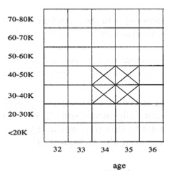
2. Dynamic discretization based on data distribution: 2D quantitative association rules: Aquan1 ^ Aquan2 => Acat (Meta rule)
각 셀에 속해 있는 수가 confidence, support가 threshold보다 높아야 한다.
3. Clustering: distance-based association
Mining interesting correlation pattern
기존의 support나 confidence는 correlation을 나타내기 좋은 도구가 아니다. 예를 들어, 전체 학생의 75%가 시리얼을 먹는데 농구를 하면 시리얼을 먹는다[40%, 66.7%]라는 rule은 의미가 없는 rule이다. confidence가 75%보다 작은 66.7%이기 때문이다. 그렇기 때문에 농구를 하지 않으면 시리얼을 먹지 않는다[20%, 33.3%]가 훨씬 의미 있는 룰이다. 결국 support와 confidence로는 역설적인 상황이 발생하기 때문에 다른 measure가 필요하게 되었다.
Corrleation을 잘 나타내기 좋은 도구로 lift, cosine, all_conf라는 것들이 있다. 그러나 강의 중엔 Lift만 다루었다.
Lift
lift = P(AUB) / P(A)*P(B)
1을 기준으로 1보다 크면 양의 상관관계이고 낮으면 음의 상관관계를 갖는다.
Constraint-based(Query-Directed) association mining
Database에 있는 모든 pattern을 찾는 것은 비현실적이다. 패턴은 너무 많기 때문에 사용자가 원하는 방향으로 mining을 진행할 수 있어야 한다. 그러려면 data mining은 interactive한 process를 가져야하며 소통에 필요한 언어인 query language가 필요한 것이다.
User flexibility : 무엇을 mining 할지 constraints를 준다.
System optimization : 효율적으로 mining 하기 위해서 constraints를 파악한다.
Constraints in Data Mining
Knowledge type constraint: classification, association, clustering etc.
Data constraint: : SQL-like 쿼리 사용 ex) 상점에서 함께 팔린 물건의 쌍을 찾아라!
Dimension/level constraint: 모든 attribute를 고려하는 것이 아닌 몇 개만 고려
Interestingness constraint: min support, min confidence에 대한 constraint 제시
Constrained Mining vs Other Operations
- Constrained Mining vs Constraint-based search
두 방법의 목표는 search space를 줄이는 것이다. 다만, constrained mining은 constraints를 만족하는 모든 패턴을 찾고, constraint-based search는 constraints를 만족하는 하나의, 일부의 답을 찾기만 하면 된다.
- Constrained Mining vs query processing in DBMS
두 방법은 해당 조건에 맞는 모든 답을 찾는 것이지만 전자는 숨겨져 있는 patterns를 찾는 것이고, 후자는 tuples을 찾는 것이다.
Constrained mining은 query processing에서 pushing selections와 유사한 철학을 공유한다. Query processing에서는 constraint와 같은 조건을 만족하지 않는 것들은 일찍이 털어낸다. 점점 처리해야 할 데이터가 줄어들어서 매우 효율적이다.
Anti-Monotonicity, Monotonicity, Succinctness for Constraint Pushing
Constraint 일찍 처리하고 싶다!! 어떻게!?!
- Anti-monotonicity: 만족하지 못하면 앞으로도 만족하지 못한다.
어떤 itemset S가 constraint에 성립하지 않으면 S의 superset도 constraint에 성립하지 않는다.
sum(S.Price) <= v 는 anti-monotone
sum(S.Price) >= v 는 not anti-monotone
range(S.profit)<=15 is anti-monotone (range는 두 값의 차이를 말한다)
- Monotonicity: 만족하면 앞으로도 만족한다.
어떤 itemset S가 constraint에 성립하면 S의 superset도 constraint에 성립한다.
sum(S.Price)>=v is monotone
min(S.Price)<=v is monotone
range(S.profit)>=15 is monotone
- Succinctness: Itemset A1이 constraint C를 만족하고, constraint C를 만족하는 모든 itemset S를 A1에 기반해서 간단히 계산해서 구할 수 있을 때, 이러한 constraint를 succinct하다고 한다.
min(S.Price)<=v is succinct
sum(S.Price)>=v is not succinct
Succinctness의 장점은 transaction database를 보지 않아도 itemset S가 어떤 item들을 선택했는지에 따라 constraint C를 만족하는지를 결정할 수 있다.
최적화: 만약 C가 succinct하면 C는 pre-counting pushable 하다. candidate-generation time에 basic elements가 포함되어있는지만 확인하면 해당 constraint를 만족하는지 확인할 수 있기 때문이다.
Converting “Tough” Constraints
tough constraints를 anti-monotone이나 monotone으로 바꾼다.
예시로, avg(S.profit)>=25와 같은 tough constraint는 item을 정렬함으로써 anti-monotone하게 바꾼다. Itemset을 <a,f,g,d,b,h,c,e>로 정렬했고, afb의 profit의 합의 평균이 25보다 작다면 afbh도 작을 것이다.
항상 뒤에 것만 추가해줄 수 있다: 정렬한 이유를 유념하자!!
Frequent-pattern mining: Summary
- Frequent pattern mining - an important task in data mining
- Scalable frequent pattern mining methods
- Apriori(Candidate generation & test)
- Projection-based(FPgrowth, CLOSET+, …)
- Vertical format approach(CHARM, …)
- Mining a variety of rules and interesting patterns
- Constraint-based mining
- Extensions and applications